Diffusion models: an introduction

Forward diffusion

In general - a diffusion process can be characterized by a Markov diffusion kernel given a final state \(\pi(x)\):

Since it’s a length-one Markov process, we have for the full joint: \[\begin{equation} q(x_{t=0:T} ) = q(x_0) \prod_{i=1}^T q(x_i | x_{i-1}) \end{equation}\]

Usually, we use a Gaussian diffusion, for which the posterior is closed form (c.f. the 1-step update in Kalman filtering):

\(\beta_i\)s are called the variance schedule, with usually \(\beta_1 < \beta_2 < ... < \beta_T\).

Moreover, due to the property of the Gaussian distribution:

\[\alpha_t := 1 - \beta_t\]

\[\bar{\alpha}_t := \prod_{s=1}^t \alpha_t\]

meaning any state in the forward process can be expressed knowing just the initial one and the variance schedule. In general, the theoretical underpinning of Langevin dynamics guarantees any smooth distribution can be corrupted into Gaussian noise, meaning the initial distribution can be almost arbitrarily complex, giving the model its expressive power.

Reverse diffusion

The reverse process is characterized by a new transition probability \(p(x)\). Its starting point is the stationary distribution at the final time \(T\):

Like before:

For Gaussian (and binomial), the joint is still in the same family; however, there is no closed-form for the parameters \(\mu\) and \(\Sigma\). These need to be estimated, in this case via neural networks.

A natural training target is the likelihood of the original data \(p(x_0)\) as given by the learned reverse process’ distribution, obtained by marginalizing the full joint: \[\begin{equation} p(x_0) = \int_{\mathcal{X}} p(x_{t=T:0}) ~ dx_1 .... dx_T \end{equation}\]

This is computationally intractable! A trick is to use annealed importance sampling - comparing the relative probability of the backward - \(p\) - and the forward trajectories \(q\), where the latter are known in closed form:

In the limit of very small \(\beta\), both directions become the same.

Variance schedule

Since \(\beta_t\) is a free parameter, it can be learned simultaneously with the whole \(K\) optimization procedure, freezing the other variables and optimizing on \(\beta\). Alternatively, the first paper also treated a sequence as a hyperparameter and used a simply linearly increasing \(\beta\). This is also the approach of Ho et al.

Estimating \(p\)

Our goal is to learn the following:

\[ p(x_{t-1} | x_t) = \mathcal{N}(\mu(x_t, t), \Sigma(x_t, t)), ~~ t \in [T, 0] \] which corresponds to estimating \(\mu(x_t, t), \Sigma(x_t, t)\).

For the variance, it is simply set to be isotropic with the diagonal entries either fixed at a constant (either \(\beta_t\) or \(\tilde{\beta}_t\)) or learned. The latter proved to be unstable in Ho et al., but has since been successfully implemented.

The mean is, of course, learned in all implementations and proceeds as follows: by inspecting the \(L_{t-1}\) term in the likelihood in Training, the minimizing mean can be expressed by the reparametrization: \[x_t = \sqrt{\bar{\alpha}_t}~x_0 + \sqrt{1 - \bar{\alpha}_t}~\epsilon \] \[\epsilon \sim \mathcal{N}(0, \mathbf{I})\]

meaning we instead learn the estimator of the noise in the mean term at step \(t\): \(\epsilon_{\theta}(x_t, t))\) from the state \(x_t\).

This can be further simplified by setting \(t\) to be continuous on \([1, T]\) and optimizing the following simplified objective for \(\epsilon_\theta(x_t, t)\):

\[\begin{equation} L_{\text{simple}}(\theta) := \mathbb{E}_{t, x_0, \epsilon} \left[\Vert \epsilon - \epsilon_\theta(\sqrt{\bar{\alpha}_t} x_0 + \sqrt{1 - \bar{\alpha}_t} \epsilon, t) \Vert^2\right] \end{equation}\] This can be optimized using standard optimization techniques, such as gradient descent. We can now state the two algorithms needed to first, train the noise estimator \(\epsilon_\theta\), and then, obtain a sample from the reverse diffusion process:

Architecture

Ho et al. used a variation of an U-net called PixelCNN++ to estimate \(\epsilon_{\theta}(x_t, t))\):

The original U-net

PixelCNN++ structure

Example - recovery

Recovery (middle row) of a spiral distribution (top) using a Gaussian diffusion model. The bottom row represents the “drift term”, i.e. the field controlling the mean for the “particles” in the next step of the reverse process.

Example - generation

Ho et al. used the modified network for both conditional and unconditional generation.

The unconditional generation was performed by estimating \(x_0\) - the end result of the reverse process - from initially random \(x_T\). The following figure shows the order in which features crystallize when the initial state is itself sampled from various points of the reverse process. The training dataset was CIFAR10.

Unconditional generation from the reverse process sample

For conditional generation, the authors selected a \(x_t\) from the actual distribution and sampled from the predictive posterior \(p(x_0|x_t)\). The following figure shows the results conditioned on the bottom-right quadrant, for a network trained on CelebA-HQ:

Conditional generation samples from a given state: the earlier the \(x_t\), the more deterministic the outcome.

Imagen & DALL-E 2

Ho and Salimans improved the above procedure by introducing the notion of guiding the model during training on labeled data, i.e. estimating \(\epsilon_\theta(x_t, t ∣ y)\), where \(y\) are the labels. The crux of the approach is training both on conditional and unconditional objectives at once by randomly setting the class label to a null class with some predetermined probability. Likewise, the samples are drawn from a convex combination (with the same coefficient) of both \(p\)-s.

This was used by Nichol et al. in GLIDE, which uses information extracted from text to do the guiding, combining a transformer with the previously described architecture.

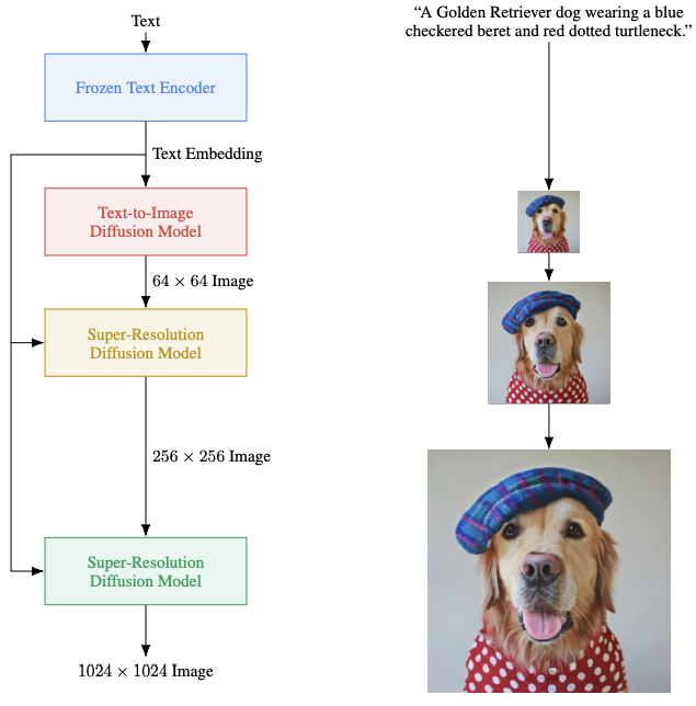
This approach has been used to construct Imagen, which uses additional diffusion models to up-sample the image created by the guided diffusion process. The text embeddings are provided by a pretrained transformer’s encoder.

Imagen structure

The other diffusion-based model to make waves recently - DALL-E 2 - uses a bit more complex approach:

DALL-E 2 architecture

First, it re-uses a model called CLIP (Contrastive Language-Image Pre-training) to construct a mapping between captions and images (top of the schematic above). In practice, the net result of this is a joint embedding of text and images in a representation space.

In generation, this model is frozen and a version of the GLIDE guided diffusion model is used to generate images starting from the image representation space (as opposed to random noise, for instance). As previously, additional up-samplers are used in the decoder, as well.

To generate from text prompts, we need to map the caption text embeddings to the above mentioned image embeddings, which are the starting point for the decoder. This is done with an additional diffusion model called the prior, which generates multiple possible embeddings. In other words, this is a generative model of the image embeddings given the text embeddings. The prior trains a decoder-only transformer to predict the conditional reverse process, as opposed to the U-net used in other examples.

DALL-E 2: interpolation of the image embedding space by the decoder

References

- The original paper: Sohl-Dickstein et al. - Deep Unsupervised Learning using Non-equilibrium Thermodynamics
- Performant implementation: Ho et al. - Denoising Diffusion Probabilistic Models
- A good blog post: Weng, Lilian. (Jul 2021). What are diffusion models? Lil’Log.
- A summary of recent developments: https://maciejdomagala.github.io/generative_models/2022/06/06/The-recent-rise-of-diffusion-based-models.html
- DALL-E 2 initial paper: Ramesh et al. - Hierarchical Text-Conditional Image Generation with CLIP Latents